Tuning an OD Process

Tuning an orbit determination process consists of adjusting a set of parameters to yield a statistically accurate estimate based on the available tracking data. Tuning can be a difficult process, but can be approached systematically by understanding the interactions of the measurement models, dynamical models, and estimation method. This guide is intended as a centralized location to discuss tuning parameters at a high level; more information on these various parameters can be found within the higher-level Setting up an OD System guide, particularly the Estimation Techniques pages for setting up different estimation methods, as well as on the object pages for each component of the OD process. Expand the list below to view relevant objects.

 Tunable OD Objects

Different tuning parameters should be adjusted for a Batch Least Squares process versus a sequential process like an Extended Kalman Filter or Square Root Information Filter. Some parameters, like the choice of estimated parameters and a priori covariance, are important to consider regardless of the estimation method.

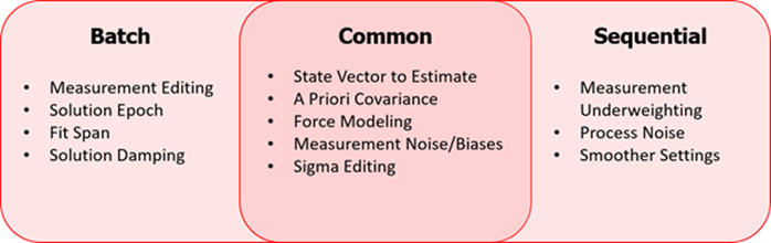
Common Tuning Parameters

Several tuning parameters can affect both types of estimation processes:

State Vector

The properties that will be estimated or considered by the process should be observable. Sometimes choice of element set can improve observability. The Equinoctial element set segments the size, shape, orientation, and location within the orbit better than the Cartesian element set. This allows for estimation of just a portion of the state vector, such as the in-plane components. Solving for a partial state vector can be helpful for weakly observable solutions with limited or sparse tracking data.

A Priori Covariance

For sequential filter processes, it is important to have a realistically sized a priori covariance to assist convergence. If the covariance is too large or too small, this can cause any type of sequential filter to diverge. If the a priori covariance is unknown, then information about the source of the a priori state should be used to provide a realistic magnitude for the covariance. Alternatively, a short-arc Batch Least Squares solution can be generated to then seed the sequential filter process with an a priori state and covariance.  

The Batch Least Squares method can be configured to handle the a priori covariance in multiple ways, including ignoring it or computing an a priori covariance based on the tracking data information. A small a priori covariance can limit the amount of state update that a Batch Least Squares estimator will apply; if that appears to be occurring, the a priori covariance could be scaled up or ignored. See Setting up a Batch Least Squares Estimator for more information.

Force Modeling

The Force Model should model the dynamics as accurately as possible. This is especially important for orbits that are heavily influenced by forces such as drag, solar radiation pressure, or gravitational perturbations. The dynamics of the orbit are an important factor for choosing an estimator type. Sequential OD processes are generally more responsive to changes in the forces acting on the spacecraft, such as atmospheric drag variation. If a Batch Least Squares estimator is desired for an orbit with variable dynamics, care should be taken to size the fit span to periodicity of the dynamical changes. See Setting up a Force Model for more information.

It is possible to estimate dynamical corrections with either a Batch Least Squares or sequential OD process. However, each process will respond to dynamical changes differently. A sequential OD process can estimate small changes to the dynamical model with each state update, whereas a Batch will estimate an average change over the entire fit-span. These corrections can be modeled through the EstimableAcceleration objects within a Spacecraft's OD properties, and should be configured like any other estimable parameter.

You also have the ability to set the Spacecraft's process noise rate information for the Cartesian element set in any natively supported Attitude Reference Frame, such as ICRF, Radial/In-Track/Cross-Track (RIC), Local Vertical/Local Horizontal( LVLH) - Earth Pointing, Velocity/Normal/Binormal (VNB), Geodetic, UVW, or a Custom Coordinate System through the SpacecraftProcessNoise object. When setting the diagonal of the process noise matrix, all off-diagonal terms of the matrix are set to zero.

Note: These methods only applies to the Cartesian Element Set for Orbit Determination. This does NOT apply to the TLE and Equinoctial Element sets.

Maneuvers are also an important consideration for the force modeling in an estimation process. Maneuvers can be modeled in all estimators and corrections can be estimated in a Batch Least Squares process, as demonstrated in the Batch Maneuver Estimation Simulate and Process sample Mission Plan. Because of maneuver execution errors, maneuvers introduce additional error into the dynamical model that must be accounted for. See the Process Noise Rate section of this guide for more information.

Measurement Noise/Biases

Measurement noise is the mechanism within an OD process to account for the random errors associated with forming a tracking data measurement. The value used should represent the true 1-sigma precision of the measurement system. Larger measurement noise values will allow more measurement data to be accepted for processing, but will reduce the amount of state-update information that the estimator extracts from the measurements. Smaller measurement noise values can cause more data to be rejected, but increases the amount of state update information from the measurements.

Measurement biases attempt to account for systemic errors in the measurement model that are not random. When possible, these biases should be modeled, but they can also be estimated. In the sequential filters, FreeFlyer treats measurement biases as a random-walk variable, and in the Batch they are treated as a constant bias over the fit span.

Sigma Editing

The sigma editing threshold can be adjusted to accept more or less data for processing. This can be opened up during tuning, but nominally should be 3-sigma. This would typically accept 99.7% of the measurement tracking data if the measurement errors are of a Gaussian distribution. This property can be edited through the MaxAllowableSigma property on either the Batch or any of the sequential filter objects. The MeasurementEditing option on the Batch Least Squares object will dictate how the sigma editing threshold is applied.

Tuning a Batch Least Squares

Tuning parameters that apply to the Batch Least Squares should be configured when setting up the Batch.

Measurement Editing

The MeasurementEditingOption property on the BatchLeastSquaresOD object lets you choose one of two different methods for performing measurement editing: use the Predicted RMS value to edit data or use the standard deviation of the measurements to edit data. The data editing threshold is scaled based on the BatchLeastSquaresOD.MaxAllowableSigma property. The Predicted RMS is computed based on an expression that uses the a priori covariance and measurement residual information. Each option behaves differently and has different applications.

The standard deviation method is a better approach when using a poor a priori state because it is able to reject outliers in the measurements, even if the measurement set as a whole is offset from the a priori trajectory. Using the Predicted RMS to edit data tends to enforce more agreement with the a priori state, and is better used when there is less uncertainty in the a priori state.

Solution Epoch

The solution epoch can be any epoch within the fit span and is typically chosen to be the beginning or end of the span. The BatchLeastSquaresOD.SolutionEpochOption allows the user to choose whether to specify an epoch or make a selection from the beginning, middle, or end of arc epochs. The choice of which to use should be informed by the contents of the state vector and knowledge of the dynamical regime.

For example, if spacecraft position, velocity, and maneuver corrections are being estimated together, the choice of solution epoch (and fit span) should ensure that there is enough pre- and post-maneuver tracking data for the Batch to estimate both parts of the state vector adequately. If the solution epoch is too close to the maneuver epoch, and there is no tracking data between the two epochs, the Batch may have problems determining whether to apply state updates to the spacecraft state or the maneuver corrections.

Fit Span

The span of the Batch Least Squares fit should be chosen as a balance between the variability of the dynamics and observability of the state estimates. The fit span can vary from single orbits for LEO satellites to multiple weeks for dynamically stable environments such as GEO or libration point orbits.

Solution Damping

Solution damping can be used to improve convergence in the Batch by reducing or "damping" the state update. There are multiple algorithms supported but each attempts to reduce the state update based on the values set and the information content in the tracking data within the Batch Least Squares fit span. This is generally only recommended in poorly observable scenarios where convergence has proven difficult.

Tuning a Filter

Tuning parameters that apply to a sequential process can be configured when setting up the process, and some can be updated dynamically as needed.

Process Noise Rate

Process noise rate is one of the primary tuning parameters for sequential filters. Process noise rate is added to covariance propagation at every time step to account for the uncertainty in the propagation models for state estimates. Larger values of process noise will provide more of an increase in uncertainty during propagation and smaller values will provide less of an increase. The magnitude of the value should reflect the expected uncertainty in the propagation model. The default reference frame for process noise corresponds to the element set chosen for the state vector.

Measurement Underweighting

Measurement underweighting is a technique to compensate for non-linear effects in the measurement data that are not accounted for in linearized measurement models. The underweighting factor reduces the state and covariance update of the filter to prevent over-tightening of the covariance, which can cause rejection of valid measurements and lead to filter divergence. This scenario is most common with very accurate measurement data and a very uncertain state vector. In this case when non-linear conditions are detected based on the measurement’s expected residuals, the underweighting factor slows down convergence of the filter.

The underweighting factor represents a ratio of the state update to use. A value of 1 does not underweight, and uses all of the state and covariance update, and a value of 0 would eliminate the state and covariance update entirely. Underweighting is available for all the sequential filter objects. However, because the Unscented Kalman Filter uses a non-linear measurement model, underweighting is not required as often.

Users can check whether or not measurement underweighting was used as part of the filter state and covariance update after an observation has been processed.

Smoother

Smoothers can be used to refine the state estimates after the forward filter pass. FreeFlyer supports multiple formulations of Smoother, and the choice of algorithm should be based on the dynamical model, the properties in the state vector and the type, accuracy, and amount of tracking data. A Smoother update is constrained by the pre- and post-update covariances, so a filter solution with a very small covariance will only achieve incremental improvements from a Smoother. More information on configuring a Smoother is available on the Setting up a Smoother page and the Using the Smoother section of the Kalman Filter, Square Root Information Filter, and Unscented Kalman Filter page.

See Also