J2 Perturbation

Top Previous Next

Long ago, people thought the Earth was flat. Many believed that you could sail to the edge of the Earth and fall off. We have long since dismissed this idea as we now know the Earth is a sphere. Right?

Actually, the Earth really isn't a sphere - it is an oblate spheroid. Because of the rotation of the Earth on its axis, centrifugal force bulges the equator. In fact, the radius at the Earth's equator is about 21 km larger than the radius at the poles. See the below diagram to understand what we're talking about:

oblateEarth

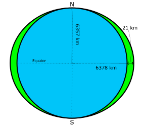
Oblate Earth

Now that we understand that our Earth is really more oblate than spherical, we need to ask ourselves some questions. How does this affect our orbits? There is a perturbing force based on this oblate Earth called "J2 Perturbations." But where does the term "J2" come from? The term J2 comes from an infinite series mathematical equation that describes the perturbational effects of oblation on the gravity of a planet. The coefficients of each term in this series is described as Jk, of which J2, J3, and J4 are called "zonal coefficients." However, J2 is over 1000 times larger than the rest and has the strongest perturbing factor on orbits.

The two main orbital elements affected by J2 Perturbations are the Right Ascension of the Ascending Node (Ω) and the Argument of Perigee (ω). If we were to model the Earth as a perfect sphere with a uniform gravitational field, the RAAN and argument of perigee would not change. But since our Earth is not really a perfect sphere, it is important that we account for this perturbation.

J2 perturbations will move the RAAN over time at a constant rate depending on the orbit's size, shape, and inclination. Using this property of J2 perturbations, we can manipulate our orbit so that the RAAN changes at a rate of 360 degrees per year, keeping the orbit in the same orientation with respect to the Sun. This is called a "Sun-Synchronous Orbit". However, if we did not account for J2, would have the red orbit in the picture below:

sunsync

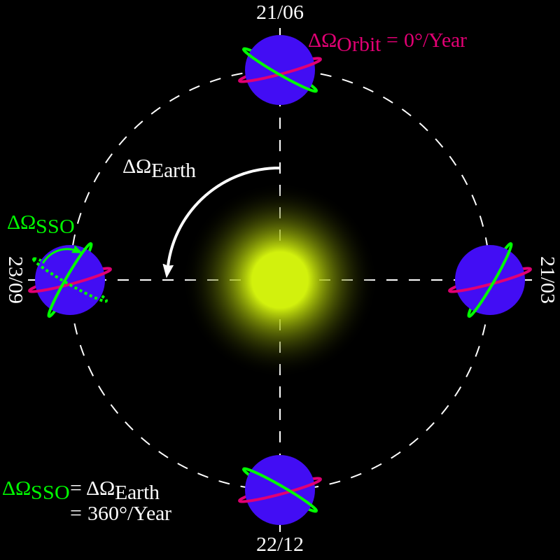
Sun-Synchronous Orbit vs Non Sun-Synchronous Orbit

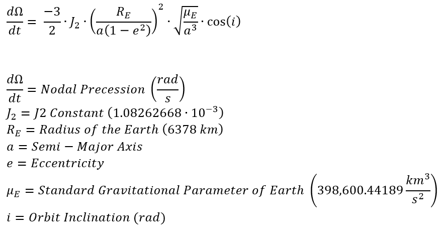
The green orbit on the other hand, does account for J2 and keeps the same orientation with respect to the Sun. The reason this is possible is because the orbit is designed to have the RAAN change 360 degrees per year. The formula for the change of RAAN over time is the formula below:

nodalPrecessionFormula

In this section, we will discuss:

1.Calculating a Sun-Synchronous Orbit

2.Modeling a Sun-Synchronous Orbit

Calculating a Sun-Synchronous Orbit

Problem:

We have a circular orbit with an SMA of 7000 km that we wish to make Sun-Synchronous. What inclination do we need for this to occur?

First, we need to calculate exactly what the nodal precession rate is. We know it needs to be 360 degrees per year, but we need to convert it to radians per seconds.

360 deg/year = 0.98562625 deg/day = 11.4077116e-6 deg/s
11.4077116e-6 deg/s = 0.19910213e-6 rad/s

Next, we need to take the formula given above and solve for the inclination. When we do that, we get this formula:

J2InclincationFormula

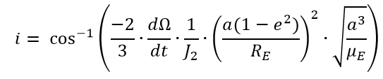
This formula looks rather complex. However, we have all of the necessary variables so let's plug in our variables and calculate the result.

a = 7000 km

e = 0

dΩ/dt = 0.19910213e-6 rad/s

J2 = 1.08262668e-3

RE = 6378.1363 km

μE= 398600.442 km^3/s^2

i = 1.7082196041 rad = 97.87377 deg

Modeling a Sun-Synchronous Orbit

Let's model the orbit whose inclination we just calculated in FreeFlyer. For demonstration purposes, we will add in a Spacecraft identical to the Sun-Synchronous Spacecraft we've calculated, but simplify the force model to a point mass and see if there is any nodal precession.

•Open a new Mission Plan and save it as "J2Perturbation.MissionPlan"

Adding in Spacecraft

•Create a new Spacecraft with the following Keplerian elements:

oA: 7000 km

oE: 0

oI: 97.87377 deg

oRAAN: 100 deg

oW: 0 deg

oTA: 0 deg

•To speed up simulation time, we will change the propagator. Go to the "Propagator" section on the left-hand side of the Spacecraft object editor

•Change the Integrator Type to "Bulirsch-Stoer VOP"

•Make sure the step mode is set to "Variable Step Size"

propagatorChange

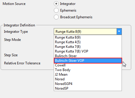
Propagator Settings in the Spacecraft Editor

•Click "Ok" to close the editor

•Right-click "Spacecraft1" and click "Clone"

•Open the newly cloned Spacecraft

•Rename it to "Spacecraft2"

•Go into "Force Model" on the left-hand side

•Change the "Field Type" to "Point Mass"

forceModelPointSource

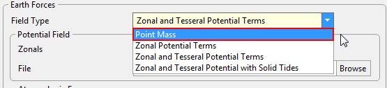
Force Model Settings in the Spacecraft Editor

•Press "Ok" to close the editor

Adding a PlotWindow

•Create a PlotWindow through the object browser

•Double-click "PlotWindow1" to open the editor

•Change the y-axis to "Spacecraft1.RAAN"

•Click "More" to add another line to the plot

•Change the new dropdown to "Spacecraft2.RAAN"

•Click "Ok" to close the editor

Building the Mission Sequence

•Drag and drop a "While...End" loop onto the Mission Sequence

•Change the argument inside the while loop to "(Spacecraft1.ElapsedTime < TIMESPAN(500 days))

•Drag and drop a FreeForm script editor inside the loop

•Change the name of the FreeForm to "Step and Update"

In this script, we will be stepping both Spacecraft with an epoch sync and updating the plot window. To do this, we write:

// Step both spacecraft with an epoch sync

Step Spacecraft1;

Step Spacecraft2 to (Spacecraft2.Epoch == Spacecraft1.Epoch);

Update PlotWindow1;

Your Mission Sequence should look something like this:

j2MS

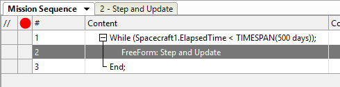
Mission Sequence Example

Save and run your Mission Plan, then try and answer these questions:

Look at the RAAN for Spacecraft1. The output should be like a saw wave. What is the period of this plot?